3D Cell visualization

In this tutorial, we will make 3D visualization of the graph components that constitute cells in MPX data using R.

Setup

library(dplyr)
library(tidyr)
library(here)
library(ggplot2)
library(pixelatorR)
library(stringr)
library(SeuratObject)

Load data

We will continue with the stimulated T cell data that we analyzed in the previous tutorial (Karlsson et al., Nature Methods 2024).

DATA_DIR <- "path/to/local/folder"
Sys.setenv("DATA_DIR" = DATA_DIR)

pg_data_combined <- readRDS(file.path(DATA_DIR, "uropod_spatial.rds"))
pg_data_combined

An object of class Seurat 
3320 features across 786 samples within 3 assays 
Active assay: colocalization (3160 features, 193 variable features)
 2 layers present: data, scale.data
 2 other assays present: mpxCells, polarization
 2 dimensional reductions calculated: pca, umap

Now we can select components with high colocalization for a specific marker pair to get some good example components to work with. First, we will filter our colocalization scores to keep only CD162/CD50 and then we will add the abundance data for CD162, CD37 and CD50 to the colocalization table.

# Make sure that we are using the correct assay
DefaultAssay(pg_data_combined) <- "mpxCells"

colocalization_scores <- 
  ColocalizationScores(pg_data_combined, meta_data_columns = "sample") %>% 
  unite(contrast, marker_1, marker_2, sep = "/") %>% 
  filter(contrast == "CD162/CD50") %>% 
  left_join(y = FetchData(pg_data_combined, vars = c("CD162", "CD50", "CD37"), layer = "counts") %>% 
              as_tibble(rownames = "component"), 
            by = "component")

Next, we will select components with high colocalization scores for CD162/CD50. In the histogram below, we see the distribution of Pearson Z scores for the CD162/CD50 colocalization. Since we want to narrow down the selection of components, we set a threshold for the Pearson Z scores. Here, we use a threshold of 35 to keep the components with the highest colocalization scores. Note that the threshold is arbitrary and should be adjusted based on the data.

# Set Pearson Z threshold
pearson_z_threshold <- 35

ggplot(colocalization_scores, aes(pearson_z)) +
  geom_histogram(bins = 50) +
  geom_vline(xintercept = pearson_z_threshold, linetype = "dashed") +
  labs(title = "Pearson Z scores [CD162/CD50]")

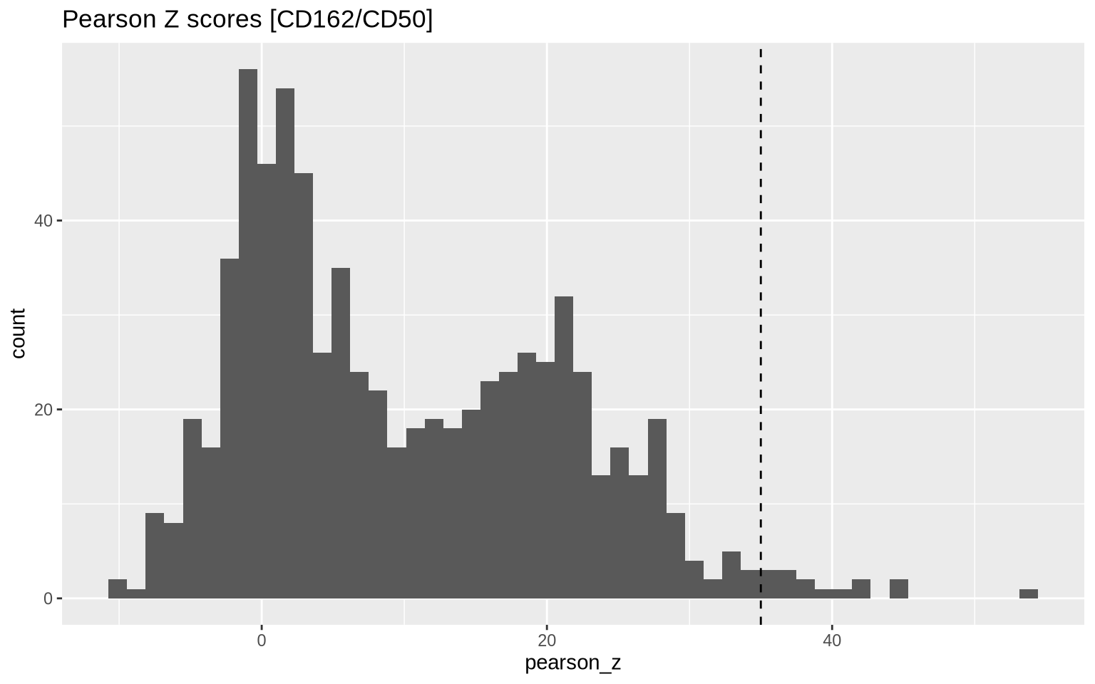
Then we apply our threshold to get a final selection of 13 components.

plot_components <- 
  colocalization_scores %>% 
  filter(pearson_z > pearson_z_threshold, sample == "Stimulated") %>% 
  arrange(-CD162) %>% 
  select(component, pearson_z, CD162, CD50, CD37)
plot_components

# A tibble: 15 × 5
   component                   pearson_z CD162  CD50  CD37
   <chr>                           <dbl> <dbl> <dbl> <dbl>
Stimulated_61cb84c709f41e7b      41.7   947  1222   631
Stimulated_59b284adcc91ec91      44.1   789   864   448
Stimulated_23606c9599265d9a      40.1   690   707   452
Stimulated_18278b69dc73ad16      41.7   486   736   249
Stimulated_437d692c40d6d601      53.8   450   493   286
Stimulated_50cd2ae85ea1c0e1      44.6   414   651   287
Stimulated_19ab7abc50018ac8      40.5   303   467   116
Stimulated_898664166bbd71ae      35.6   301   626   317
Stimulated_d33f7aa55f7874ff      36.5   220   238   112
Stimulated_7778298975953f4f      36.9   216   420   138
Stimulated_703a192bee0b36f2      38.0   197   183   178
Stimulated_f4d9b2d31012177a      38.4   178   161   119
Stimulated_bd77e6c5f6e229e5      36.7   153   289   108
Stimulated_60523a26c6f19593      35.9   136   111    38
Stimulated_8a91a136efcae912      35.4    68   118    69

Visualize single cell graph components in 3D

As one of the main features of the MPX technology, we can create three-dimensional layouts to visualize single cells. The layout algorithms wpmds and fr that we used in 2D Cell Visualization can also be used here.

Pre-computed layouts

As we learned in the 2D visualization tutorial, we can use pre-computed layouts if they are available in our PXL files. Alternatively, we use the ComputeLayout method to generate 3D layouts after we have loaded our component graphs with LoadCellGraphs. For the latter option, we need to set dim = 3 to make sure that the layout is computed in 3D:

# Run this to load graphs and compute 3D layouts
pg_data_combined <- pg_data_combined %>% 
  LoadCellGraphs(cells = plot_components %>% 
                   pull(component)) %>% 
  ComputeLayout(dim = 3, layout_name = "wpmds")

In this tutorial, we load the pre-computed layouts from the PXL files.

pg_data_combined <- pg_data_combined %>% 
  LoadCellGraphs(cells = plot_components %>% 
                   pull(component),
                 force = TRUE,
                 load_layouts = TRUE)

Now when we have the 3D layouts, we can visualize component graphs as 3D scatter plots where each point corresponds to a UPI. Just as in the 2D plots, we can color the points based on marker abundance to see how it is distributed on the cell surface. However, now that we have a 3D layout, we get an interactive plot that we can rotate, pan and zoom. Since the 3D scatter plots are quite complex, Plot3DGraph only displays the layout for a single component.

From our table above, we can select any component. The “Stimulated_RCVCMP0001141” cell is a good candidate to visualize in 3D as it has a high Pearson Z score for CD162/CD50 and high abundance of CD162, CD50 and CD37. If we project the abundance of one of the uropod markers (CD162) on the nodes, we see that counts are indeed clustered to a small area of the cell surface.

Plot3DGraph(pg_data_combined, 
            cell_id = "Stimulated_898664166bbd71ae",
            marker = "CD162", 
            layout_method = "wpmds_3d", node_size = 3,
            colors = colorRampPalette(colors = c("gray80", "orangered"))(20)) %>% 
  plotly::layout(scene = list(xaxis = list(title = "", showgrid = F, nticks = 0, showticklabels = F),
                      yaxis = list(title = "", showgrid = F, nticks = 0, showticklabels = F),
                      zaxis = list(title = "", showgrid = F, nticks = 0, showticklabels = F)))

We can also normalize the 3D coordinates to a unit sphere.

Plot3DGraph(pg_data_combined, 
            cell_id = "Stimulated_RCVCMP0001141",
            marker = "CD162", 
            layout_method = "wpmds_3d", node_size = 3,
            project = TRUE,
            colors = colorRampPalette(colors = c("gray80", "orangered"))(20)) %>% 
  plotly::layout(scene = list(xaxis = list(title = "", showgrid = F, nticks = 0, showticklabels = F),
                      yaxis = list(title = "", showgrid = F, nticks = 0, showticklabels = F),
                      zaxis = list(title = "", showgrid = F, nticks = 0, showticklabels = F)))

Viewing colocalization of markers

We can also visualize the colocalization of two markers in 3D. Here, we visualize CD162 and CD50 on the same MPX cell component. We use the same approach as above, but now we create two plots and combine them in one view.

# Create a plot for CD162
plotly_obj_cd162 <- Plot3DGraph(pg_data_combined, 
            cell_id = "Stimulated_898664166bbd71ae",
            marker = "CD162", 
            layout_method = "wpmds_3d", node_size = 3,
            colors = colorRampPalette(colors = c("gray80", "orangered"))(20),
            scene = "scene") %>% 
  plotly::colorbar(x = -0.1, y = 1) %>% 
  plotly::layout(title = list(title = ''))
plotly_obj_cd162$x$layout$annotations <- NULL

# Create a plot for CD50
plotly_obj_cd50 <- Plot3DGraph(pg_data_combined, 
            cell_id = "Stimulated_898664166bbd71ae",
            marker = "CD50", 
            layout_method = "wpmds_3d", node_size = 3,
            colors = colorRampPalette(colors = c("gray80", "orangered"))(20),
            scene = "scene2") %>% 
  plotly::colorbar(y = 1)
plotly_obj_cd50$x$layout$annotations <- NULL

# Combine plots
main_plot <- plotly::subplot(plotly_obj_cd162, 
                     plotly_obj_cd50, nrows = 1, margin = 0.06) %>% 
  plotly::layout(scene = list(domain = list(x = c(0, 0.5), 
                      aspectmode = "cube")), 
         scene2 = list(domain = list(x = c(0.5, 1), 
                      aspectmode = "cube"))
  ) %>% 
  plotly::hide_legend()

main_plot$x$layout[1:2] <- NULL

# Add marker annotations
annotations = list(
  list(
    x = 0.2,
    y = 1.0,
    text = "CD162",
    xref = "paper",
    yref = "paper",
    xanchor = "center",
    yanchor = "bottom",
    showarrow = FALSE
  ),
  list(
    x = 0.8,
    y = 1,
    text = "CD50",
    xref = "paper",
    yref = "paper",
    xanchor = "center",
    yanchor = "bottom",
    showarrow = FALSE
  )
)

main_plot <- main_plot %>% plotly::layout(annotations = annotations) 

# We can sync the plots with some custom JavaScript code
main_plot %>% 
  htmlwidgets::onRender(
    "function(x, el) {
      x.on('plotly_relayout', function(d) {
        const camera = Object.keys(d).filter((key) => /\\.camera$/.test(key));
        if (camera.length) {
          const scenes = Object.keys(x.layout).filter((key) => /^scene\\d*/.test(key));
          const new_layout = {};
          scenes.forEach(key => {
            new_layout[key] = {...x.layout[key], camera: {...d[camera]}};
          });
          Plotly.relayout(x, new_layout);
        }
      });
    }")

Setup​

Load data​

Visualize single cell graph components in 3D​

Pre-computed layouts​

Viewing colocalization of markers​

Setup

Load data

Visualize single cell graph components in 3D

Pre-computed layouts

Viewing colocalization of markers